Generating uniformly distributed numbers on a sphere

So, we want to generate uniformly distributed random numbers on a unit sphere. This came up today in writing a code for molecular simulations. Spherical coordinates give us a nice way to ensure that a point $(x,y,z)$ is on the sphere for any $(\theta,\phi)$ :

$x = r \sin(\phi) \cos(\theta)$ $y = r \sin(\phi) \sin(\theta)$ $z = r \cos(\phi).$

In spherical coordinates, $r$ is the radius, $\theta \in [0,2\pi]$ is the azimuthal angle, and $\phi \in [0,\pi]$ is the polar angle.

A tempting way to generate uniformly distributed numbers in a sphere is to generate a uniform distribution of $\theta$ and $\phi$ , then apply the above transformation to yield points in Cartesian space $(x,y,z)$ , as with the following C++ code.

#include<random>
#include<cmath>
#include<chrono>

int main(int argc, char *argv[]) {
    // Set up random number generators
    unsigned seed = std::chrono::system_clock::now().time_since_epoch().count();
    std::mt19937 generator (seed);
    std::uniform_real_distribution<double> uniform01(0.0, 1.0);

    // generate N random numbers
    int N = 1000;

    // the incorrect way
    FILE * incorrect;
    incorrect = fopen("incorrect.csv", "w");
    fprintf(incorrect, "Theta,Phi,x,y,z\n");
    for (int i = 0; i < N; i++) {
        // incorrect way
        double theta = 2 * M_PI * uniform01(generator);
        double phi = M_PI * uniform01(generator);
        double x = sin(phi) * cos(theta);
        double y = sin(phi) * sin(theta);
        double z = cos(phi);
        fprintf(incorrect, "%f,%f,%f,%f,%f\n", theta, phi, x, y, z);
    }
    fclose(incorrect);
}

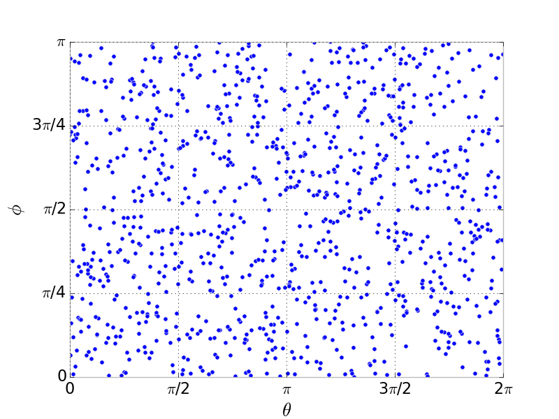
The distribution in the $\theta$ - $\phi$ plane in this strategy is uniform:

After mapping these points in the $\theta$ - $\phi$ plane to the sphere using the relationship between spherical and Cartesian coordinates above, this incorrect strategy yields the following distribution of points on the sphere. We see that the points are clustered around the poles ( $\phi=0$ and $\phi=\pi$ ) and sparse around the equator ( $\phi=\pi/2$ ).

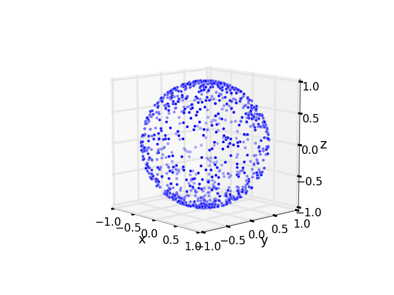
The reason for this is that the area $dA$ of a differential surface element in spherical coordinates is $dA(d\theta, d\phi) =r^2 \sin (\phi) d\phi d\theta$ . This formula for the area of a differential surface element comes from treating it as a square of dimension $r d\phi$ by $r \sin(\phi)d\theta$ . These dimensions of the differential surface element come from simple trigonometry.

So, close to the poles of the sphere ( $\phi=0$ and $\phi=\pi$ ), the differential surface area element determined by $d\theta$ and $d\phi$ gets smaller since $\sin(\phi)\rightarrow 0$ . Thus, we should include less points near $\phi=0$ and $\phi=\pi$ and more points near $\phi=\pi/2$ to achieve a uniform distribution on the sphere.

Our goal is to find and then draw samples from the probability distribution $f(\theta, \phi)$ that maps from the $\theta$ - $\phi$ plane to a uniform distribution on the sphere.

Let $v$ be a point on the unit sphere $S$ . We want the probability density $f(v)$ to be constant for a uniform distribution. Thus $f(v) = \frac{1}{4\pi}$ since $\int \int_S f(v) dA = 1$ and $\int \int_S dA = 4\pi$ . We want to represent points $v$ using the parameterization in $\theta$ and $\phi$ and find the corresponding probability density function $f(\theta, \phi)$ that maps to a uniform distribution on the sphere. We can obtain a uniform distribution by enforcing:

$f(v) dA = \frac{1}{4\pi} dA = f(\theta, \phi)d\theta d\phi,$

since $f(v)dA$ is the probability of finding a point in an area $dA$ about $v$ on the sphere. Because $dA = \sin (\phi) d\phi d\theta$ , it follows that $f(\theta, \phi) = \frac{1}{4\pi} \sin(\phi)$ .

Marginalizing the joint distribution to get the p.d.f of $\theta$ and $\phi$ separately:

$f(\theta) = \int_0^{\pi} f(\theta, \phi) d\phi = \frac{1}{2\pi}$ $f(\phi) = \int_0^{2\pi} f(\theta, \phi) d\theta = \frac{\sin(\phi)}{2}.$

We see that $\theta$ is a uniformly distributed variable and $f(\phi)$ scales with $\sin(\phi)$ ; we want more points around the equator, $\phi = \pi/2$ , which is where $\sin(\phi)$ takes its maximum.

Now, how can we sample numbers $\phi$ that follow the distribution $f(\phi)$ ? We’d like to use the readily available uniform random number generator in $[0,1]$ as before. Inverse Transform Sampling is a method that allows us to sample a general probability distribution using a uniform random number. For this, we need the cumulative distribution function of $\phi$ :

$F(\phi) = \int_0^\phi f(\hat{\phi})d\hat{\phi} = \frac{1}{2} (1-\cos(\phi)).$

Keep in mind that $F(\phi)$ is a monotonically increasing function from $[0,\pi]\rightarrow[0,1]$ since it is a cumulative distribution function. Thus, it has an inverse function $F^{-1}$ .

Let $U$ be the uniform random number in $[0,1]$ that we do know how to generate. To see how inverse transform sampling works, note that

$Pr(U \leq F(\phi))=F(\phi).$

This is a property of the uniform random variable $U[0,1]$ , since for any number $x\in[0,1]$ , $Pr(U\leq x)=x$ . As $F$ is invertible and monotone, we can preserve this inequality by writing:

$Pr(F^{-1}(U)\leq\phi)=F(\phi).$

Aha! This shows that $F(\phi)$ is the cumulative distribution function for the random variable $F^{-1}(U)$ ! Thus, $F^{-1}(U)$ follows the same distribution as $\phi$ . The algorithm for sampling the distribution $f(\phi)$ using inverse transform sampling is then:

Generate a uniform random number $u$ from the distribution $U[0,1]$ .
Compute $\phi$ such that $F(\phi) = u$ , i.e. $F^{-1}(u)$ .
Take this $\phi$ as a random number drawn from the distribution $f(\phi)$ .

In our case, $F^{-1}(u) = \arccos(1-2u)$ .

The algorithm below in C++ shows how to generate uniformly distributed numbers on the sphere using this method:

#include<random>
#include<cmath>
#include<chrono>

int main(int argc, char *argv[]) {
    // Set up random number generators
    unsigned seed = std::chrono::system_clock::now().time_since_epoch().count();
    std::mt19937 generator (seed);
    std::uniform_real_distribution<double> uniform01(0.0, 1.0);

    // generate N random numbers
    int N = 1000;

    // the correct way
    FILE * correct;
    correct = fopen("correct.csv", "w");
    fprintf(correct, "Theta,Phi,x,y,z\n");
    for (int i = 0; i < N; i++) {
        // incorrect way
        double theta = 2 * M_PI * uniform01(generator);
        double phi = acos(1 - 2 * uniform01(generator));
        double x = sin(phi) * cos(theta);
        double y = sin(phi) * sin(theta);
        double z = cos(phi);
        fprintf(correct, "%f,%f,%f,%f,%f\n", theta, phi, x, y, z);
    }
    fclose(correct);
}

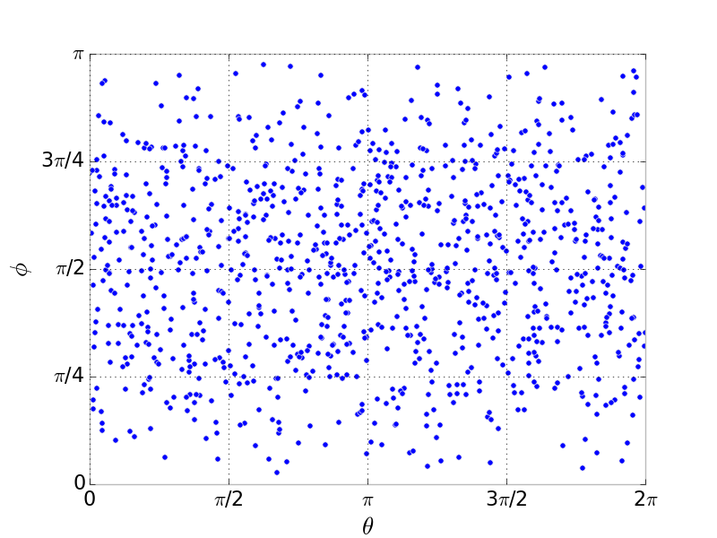
We then get the following distribution of points in the $(\theta, \phi)$ plane. There are more points around $\phi=\pi/2$ (the equator) than around the poles ( $\phi = 0, \pi$ ), as we had hoped for.

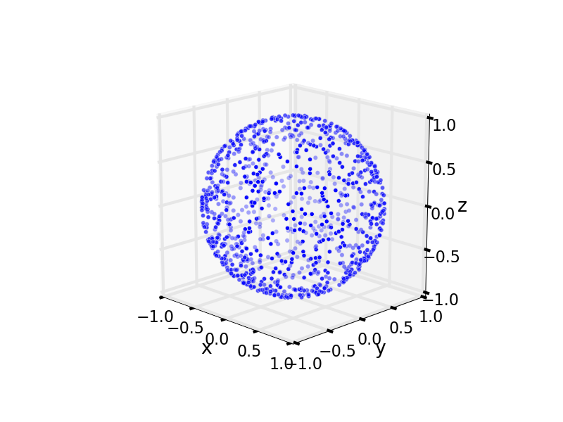
And, finally, a uniform distribution of points on the sphere.

Alternative method 1

An alternative method to generate uniformly disributed points on a unit sphere is to generate three standard normally distributed numbers $X$ , $Y$ , and $Z$ to form a vector $V=[X,Y,Z]$ . Intuitively, this vector will have a uniformly random orientation in space, but will not lie on the sphere. If we normalize the vector $V:=V/\|V\|$ , it will then lie on the sphere.

The following Julia code implements this. We have to be careful in the case that the vector has a norm close to zero, in which we must worry about floating point precision by dividing by a very small number. This is the reason for the while loop.

n = 100

f_normal = open("normal.csv", "w")
write(f_normal, "x,y,z\n")

for i = 1:n
    v = [0, 0, 0]  # initialize so we go into the while loop

    while norm(v) < .0001
        x = randn()  # random standard normal
        y = randn()
        z = randn()
        v = [x, y, z]
    end
    
    v = v / norm(v)  # normalize to unit norm

    @printf(f_normal, "%f,%f,%f\n", v[1], v[2], v[3])
end

To prove this, note that the standard normal distribution is:

$f(x) = \frac{1}{\sqrt{2\pi}}e^{- \frac{1}{2}x^2}.$

As $X$ , $Y$ , and $Z$ each follow the standard normal distribution and are generated independently:

$f(x,y,z)=f(v)= \left(\frac{1}{\sqrt{2\pi}}e^{- \frac{1}{2}x^2} \right) \left(\frac{1}{\sqrt{2\pi}}e^{- \frac{1}{2}y^2} \right) \left(\frac{1}{\sqrt{2\pi}}e^{- \frac{1}{2}z^2} \right).$

With some algebra:

$f(x,y,z)=f(v)= \frac{1}{(2\pi)^\frac{3}{2}}e^{- \frac{1}{2}(x^2+y^2+z^2)} = \frac{1}{(2\pi)^\frac{3}{2}}e^{- \frac{1}{2}\|v\|^2}.$

This shows that the probability distribution of $v$ only depends on its magnitude and not any direction $\theta$ and $\phi$ . The vectors $v$ are thus indeed pointing in uniformly random directions. By finding where the ray determined by this vector $v$ intersects the sphere, we have a sample from a uniform distribution on the sphere.

Alternative method 2

Credit to FX Coudert for pointing this out in a comment, another method is to generate uniformly distributed numbers in the cube $[-1,1]^3$ and ignore any points that are further than a unit distance $r$ from the origin. This will ensure a uniform distribution in the region $r \leq 1$ . Next, normalize each random vector to have unit norm so that the vector retains its direction but is extended to the sphere of unit radius. As each vector within the region $r\leq1$ has a random direction, these points will be uniformly distributed on a sphere of radius 1.

Alternative method 1 can be used to efficiently generate uniformly distributed numbers on a hypersphere– i.e. in higher dimensions. On the other hand, as the number of dimensions grows, the ratio of the volume of the edges of a cube to the volume of the ball inside of it grows (see Wikipedia article). Hence, a larger and larger fraction of the uniformly generated numbers in the cube will be rejected using Alternative method 2, and so this algorithm will be inefficient.

Mathemathinking

Math, Data, Machine learning, Chemical engineering

Generating uniformly distributed numbers on a sphere

Alternative method 1

Alternative method 2