By Cory Simon and Bernard Konrad

In light of the recent ebola outbreak, we have many questions about the spread of ebola that are mathematical in nature: How many people will be infected from Ebola if the disease continues to propagate? If a plane arrives with \(x\) ebola cases that mix into the population, how large must \(x\) be such an epidemic will ensue? What extent of quarantining is required to subdue the outbreak? Mathematical models attempt to answer such questions by quantifying the dynamics of disease transmission. These models are helpful in guiding policy decisions and efficiently allocating resources to mitigate the outbreak.

The Centers for Disease Control and Prevention (CDC) recently used a mathematical model to extrapolate the ebola epidemic and projected that Liberia and Sierra Leone will have had 1.4 million ebola cases by Jan. 20, 2015 in a business-as-usual scenario. Here, we will intuit the mathematics that are involved in making such an extrapolation.

The CDC’s model is an extension of the classical SIR model developed by Kermack and McKendrick in 1927 [2]. The SIR model is a compartmental model; we consider each individual of the population to be in one of three compartments: Susceptible, Infectious, and Recovered. Susceptible individuals can catch ebola from coming into contact with the infectious individuals. Infectious individuals will eventually recover, where they cannot contract ebola again nor infect susceptibles; here, recovered individuals include those who die from the disease¹. We visualize the flow of individuals through the compartments as:

The CDC model adds an additional compartment, Incubating, to take into account that individuals can be infected with ebola but are not yet contagious (infectious). An individual infected with ebola is not contagious until he or she exhibits symptoms, and this SIIR (extra “I”) model allows us to distinguish between the different interactions of susceptibles with the infected and infectious. For parsimony, we will carry on with analyzing the SIR model.

Let the variables \(S(t)\), \(I(t)\), and \(R(t)\) be the number of people in the given compartment at any time \(t\). One of our goals is to extrapolate the ebola outbreak by predicting what \(I(t)\) will look like. i.e., to generate a graph such as below that predicts how many people will be infected and how fast the epidemic will spread.

The mathematical machinery that we use to model the movement/flow of individuals from the Susceptible to Infectious to Recovered compartments is a differential equation. In a differential equation, we write the rate at which these movements occur. For example, \(dI(t)/dt\) is the number of individuals per unit time that are becoming infectious with ebola at time t.

The SIR model describes simple rules for how \(S(t)\), \(I(t)\), and \(R(t)\) will behave through modeling with differential equations, rather than prescribing an actual function form. This is natural for two reasons. First, we know how long an individual stays infectious with ebola and thus the expected residence time of an individual in the infectious compartment. Second, we know that, qualitatively, the rate at which ebola is transmitted depends on how many infectious individuals are around and the degree of mixing/interaction of them with susceptible individuals.

Let’s build and intuit the differential equations that govern the rate of change of \(S(t)\), \(I(t)\), and \(R(t)\), the SIR model.

The rate of change of the susceptible population is negative since, as ebola propagates, susceptibles leave their compartment and enter the infectious one. If there are many infectious individuals around, there are more opportunities for contact between the susceptibles and infectious and thus ebola will spread more quickly. Similarly, the more susceptibles around, the more opportunity for a given infectious individual to transmit the virus. For these intuitive reasons, the rate at which people leave the susceptible category (and become infectious) is proportional to the product of \(I(t)\) and \(S(t)\):

The parameter \(\beta\) encapsulates two pieces of information: (i) how easily the virus is transmitted and (ii) the rate of mixing/contact between susceptible and infectious individuals². Comparing to influenza, which can be transmitted through the air, ebola is not as easily transmitted and thus \(\beta\) is lower. If the population in question is a nightclub (rural Kansas), \(\beta\) is quite high (low). The quarantine policy is also embedded in parameter \(\beta\): \(\beta\) will decrease if we try to limit the infectious from interacting with susceptibles, and this is a crude way to model a quarantine policy.

As susceptibles that become infected enter the infectious category, the same mixing term appears in the differential equation for the infectious category but with a positive sign to represent an increase instead of decrease:

The additional term \(\gamma I(t)\) represents the infectious individuals recovering from the disease or dying, and thus leaving the infectious compartment (hence, the minus sign). The parameter encapsulates how long an individual spends in the infectious category; can be taken directly from studies that show how long an individual with ebola is infectious (6 days [1], so \(\gamma = \) 1/6 days\(^{-1}\)). A disease like HIV will have a very low \(\beta\) because individuals with HIV are infectious for their lifetime.

The differential equation for the recovered individuals³ collects the infectious individuals that left that category:

To put it all together, we write the entire SIR model here:

Models of similar flavor to that used by the CDC for ebola are used to model the transmission of other diseases, such as influenza, HIV, and measles.

Say we inject a few infectious individuals into a population and simulate the SIR model. Mathematically, this is imposing an initial condition to the set of differential equations above. The model allows for two separate cases:

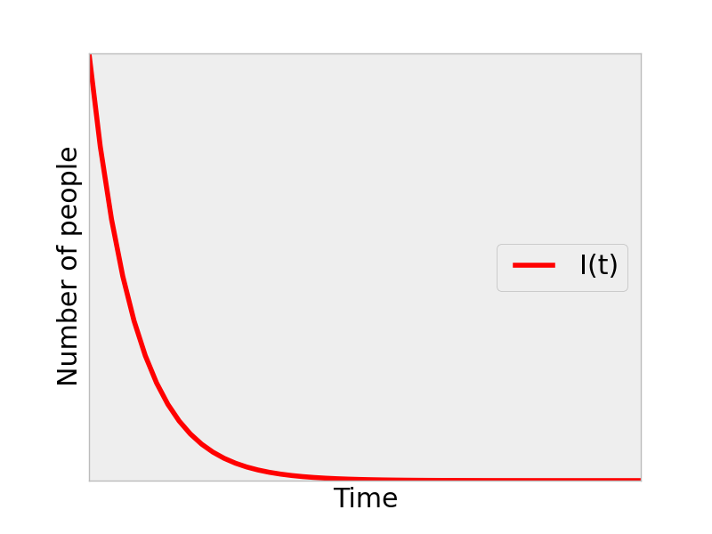
1. Ebola dies off: the infectious population decays monotonically to zero

2. An epidemic starts: the infectious population peaks and eventually drops off.

Intuitively, a large enough \(\beta\) parameter, which represents an easily-transmitted virus and/or a fast-mixing population, would lead to scenario 2. Similarly, if infectious individuals are infections for a long time (small \(\gamma\)), then a given infectious individual has a greater chance to pass on the disease and a epidemic is more likely to ensue. This is somewhat paradoxical: the most virulent diseases are less prone to a epidemic because the infectious die off quickly and have less time to transmit the disease.

We can write a computer program (e.g. open-source Scipy) to approximate the solution to these differential equations and arrive at a prediction of the progression of the ebola outbreak with time.

For an example of scenario 1 above, we set \(\beta\) to be a low value and plotted \(I(t)\):

For a more interesting example, we bumped up \(\beta\):

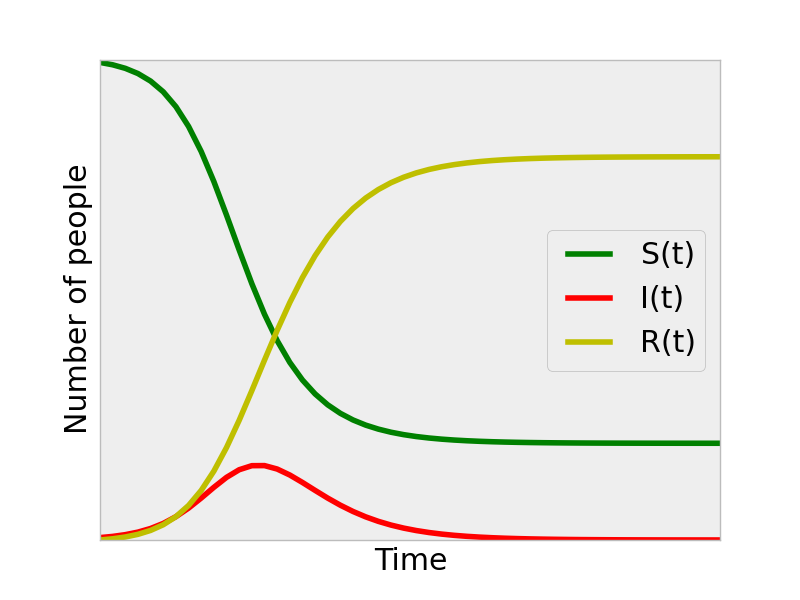
We see that an epidemic ensues and arrive at a prediction for how the outbreak will progress; the number of infectious individuals increases from the initial condition, peaks, and then drops off. Looking at the \(S(t)\) curve, we can see the prediction of what fraction of the population will be infected by the end of the outbreak for these \(\beta,\gamma\) SIR parameters. Note that the entire population was not infected. This is because the transmission of the disease lost its momentum as less susceptible individuals were around to get infected as the outbreak progressed. Analogous to combustion, the fuel (infectious) runs out of oxygen (susceptibles), and the fire ceases even though there is still fuel left.

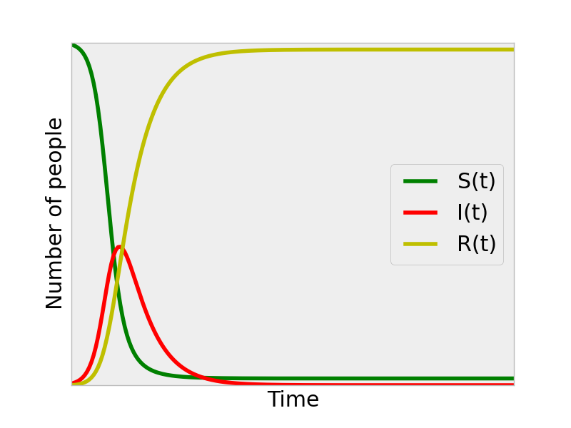
If we set \(\beta\) to be even larger, to represent a faster mixing population and more easily-transmitted virus, we see that we reach a peak in infectious individuals sooner, and, at the end of the epidemic, a greater fraction of the population has been infected (there are almost no susceptibles left at the end of this simulation.).

This is a flavor of how the CDC extrapolated the ebola epidemic to arrive at the prediction that Liberia and Sierra Leone will have had 1.4 million ebola cases by Jan 20, 2014. Given that we already have the beginning of the \(I(t)\) curve for these countries, we can identify the \(\beta\) parameter that fits the data best, and use this \(\beta\) [and \(\gamma\) from how long one stays infectious] to extrapolate the outbreak.

Remark on modeling the mixing of infectious and susceptible individuals

Essentially, all models are wrong, but some are useful. -George Box

Consider again our simple equation for the rate at which susceptibles get infected:

In chemical engineering, we use the same equation to model the time-evolution of the concentration of two chemical species \(S\) and \(I\) as they react together in a well-mixed container. Imagine \(S\) and \(I\) diffusing around (undergoing a random walk) in the container; a pair of \(S\) and \(I\) molecules only have a chance to react when they happen to collide with each other. Thus, a greater concentration of S molecules in solution, the more likely a given I molecule will collide with it, and visa versa. This is analogous to the way we model the mixing of infectious individuals coming into contact (colliding) and infecting (reacting) the susceptibles. Thus, the equation above simplifies the complex, heterogeneous contact network of our society and assumes a homogenous mixing between the susceptible and infectious individuals in the population. Literally, like we are two molecules floating around in a glass of water. This is obviously a crude approximation, but such a simple model can sometimes give surprisingly reasonable results.

Other groups have incorporated more fancy contact schemes and even agent-based models where each individual is tracked separately.

Footnotes

¹ Ebola is interesting in that dead bodies are still transmitting the virus because of the burial practices in some countries in Africa. The CDC report acknowledges this and includes dead bodies that have not yet been properly buried/cremated in the Infectious category.

² In our paper, Nino and I teased out the effects of ease of transmission of the virus and the rate of contact between susceptibles and infectious in an age-structured model for influenza.

³ The differential equation for \(R(t)\) is redundant at this point since an individual not in S or I is necessarily in R. One can see that the population is conserved in the SIR model by adding together the number of people in all compartments and taking the derivative with respect to time: \(d/dt (S+I+R)=0\), indicating that the population (\(=S+I+R\)) does not increase or decrease in this model (pedantically, assuming that someone who has died from the disease is still a member of the population).

References

[1] taken from CDC report, which references two irrelevant references… (?)

[2] Kermack, W. O.; McKendrick, A. G. (1927). “A Contribution to the Mathematical Theory of Epidemics”. Proceedings of the Royal Society A: Mathemtical, Physical and Engineering Sciences 115 (772): 700.

Python Code

import numpy as np
from scipy.integrate import odeint
import matplotlib.pyplot as plt


# SIR model parameters
N = 1.0 # population (normalized)
b = 2.0 # \beta
g = 1.0 # \gamma

def RHS(y, t):
    """
    Right hand side of SIR ODE
    y = [S(t), I(t), R(t)]
    returns derivative at (y, t)
    """
    z = np.zeros((3,))
    z[0] = -b * y[0] * y[1]/ N
    z[1] = b * y[0]* y[1]/ N - g * y[1]
    z[2] = g * y[1]
    return z

# initial condition
y0 = np.array([0.995, 0.005, 0.0])
# solve on this array of times
t = np.linspace(0, 20, 200)
# solve ODE
y = odeint(RHS, y0, t)

# plot results
fig = plt.figure()
plt.plot(t, y[:,0], label='S(t)', color='g')
plt.plot(t, y[:,1], label='I(t)', color='r')
plt.plot(t, y[:,2], label='R(t)', color='y')
plt.xticks([])
plt.yticks([])
plt.xlabel('Time')
plt.ylabel('Number of people')
plt.legend(loc='center right')
plt.savefig('sir.png', format='png')
plt.show()