Julia is a young dynamic programming language for technical computing with reads-like-a-book syntax similar to Python but speed that approaches that of C in many cases. In this post, I will illustrate how you can exploit a multi-core processor on your laptop or desktop computer by parallelizing code in Julia.

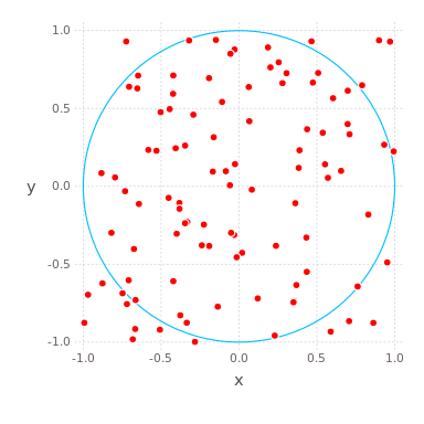
As an embarassingly parallel algorithm for an example, we will compute \(\pi=3.14159265…\), the ratio of a circle’s circumference to its diameter, using a Monte Carlo simulation. It follows from the definition of \(\pi\) that the area of a circle is \(A=\pi r^2\), where \(r\) is the radius of a circle. We can develop a Monte Carlo algorithm to compute \(\pi\) by randomly throwing darts– i.e. generating uniformly distributed random numbers in a box \([-1,1]^2\) in the \(x\)-\(y\) plane and counting the fraction of the points that land inside the circle.

As the ratio of the area of the circle (\(A=\pi\), since \(r=1\) here) to that of the square (\(A=4\)) is \(\pi /4\), this should be equal to the fraction of points that land in the circle if we throw an infinite number of random darts in this box. Thus, our estimate of \(\pi\) is four times the fraction of points that land in the circle.

Below is a function compute_pi(N) in Julia that computes an estimate of \(\pi\) using \(N\) Monte Carlo darts, written in serial code.

function compute_pi(N::Int)
    """
    Compute pi with a Monte Carlo simulation of N darts thrown in [-1,1]^2
    Returns estimate of pi
    """
    n_landed_in_circle = 0  # counts number of points that have radial coordinate < 1, i.e. in circle
    for i = 1:N
        x = rand() * 2 - 1  # uniformly distributed number on x-axis
        y = rand() * 2 - 1  # uniformly distributed number on y-axis

        r2 = x*x + y*y  # radius squared, in radial coordinates
        if r2 < 1.0
            n_landed_in_circle += 1
        end
    end

    return n_landed_in_circle / N * 4.0    
end

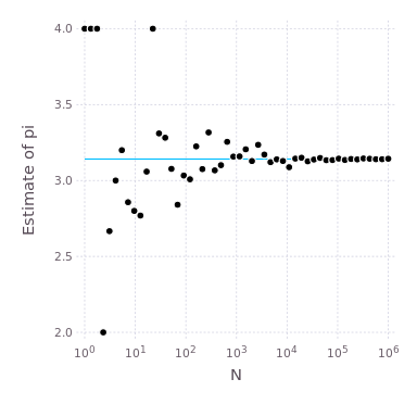
As we throw more and more darts, the estimate should converge to the value of \(\pi\) within machine precision, assuming the random number generator is perfect. The plot below shows how the estimate of \(\pi\) gets better as we increase the number of darts, \(N\). The blue, horizontal line is the true value of \(\pi\). Note the log scale on the \(x\)-axis.

The process of throwing darts and counting the fraction that land in the circle is embarassingly parallel: each dart is completely independent of the other darts thrown. So, if I want 8 billion Monte Carlo samples to get a really good estimate of \(\pi\), I can assign each of the 8 cores on my CPU to throw 1 billion darts in parallel to speed up the computation. Each core will run the compute_pi(1000000000) function in parallel. After all of the cores finish, I can add up the number of darts that landed inside the circle for each core. The statistical quality of the Monte Carlo estimate of \(\pi\) that we get with this parallelized algorithm is equivalent to that of the serial algorithm that sequentially throws 8 billion darts in a row. The analogy is that, if I need to flip a coin 800 times and count the fraction of heads, I can recruit 7 of my friends to help. If we all flip the coin 100 times, we get the same quality result, but we can get the job done faster since we can all flip our coins at once.

In the shell, start Julia using all 8 cores¹:

Now, within Julia, we need to tell all 8 cores about the function compute_pi(N), which we can do with the @everywhere macro.

@everywhere function compute_pi(N::Int)
    """
    Compute pi with a Monte Carlo simulation of N darts thrown in [-1,1]^2
    Returns estimate of pi
    """
    n_landed_in_circle = 0  # counts number of points that have radial coordinate < 1, i.e. in circle
    for i = 1:N
        x = rand() * 2 - 1  # uniformly distributed number on x-axis
        y = rand() * 2 - 1  # uniformly distributed number on y-axis

        r2 = x*x + y*y  # radius squared, in radial coordinates
        if r2 < 1.0
            n_landed_in_circle += 1
        end
    end

    return n_landed_in_circle / N * 4.0    
end

To spawn a remote call on an available core, we can use the @spawn macro.

A remote call is a request by one process to call a certain function on certain arguments on another (possibly the same) process. A remote call returns a remote reference to its result. Remote calls return immediately; the process that made the call proceeds to its next operation while the remote call happens somewhere else.

-- Julia docs

We then fetch the result, which is the estimate of \(\pi\) on that particular core using 1 billion Monte Carlo samples.

job = @spawn compute_pi(1000000000)
fetch(job)

We’d like to spawn this Monte Carlo simulation of 1 billion darts on all 8 cores and take the average estimate of \(\pi\), which is the same quality estimate of running the serial code with 8 billion darts. Instead of using the @spawn macro ourselves, Julia has syntax for distributing these jobs to the cores in a for loop and performing a reduction, which is a parallel programming term for combining the result from multiple cores. The reduction we want to perform is an addition. At the end, we divide by the number of cores to get the average estimate of \(\pi\) among the cores.

function parallel_pi_computation(N::Int; ncores::Int=8)
    """
    Compute pi in parallel, over ncores cores, with a Monte Carlo simulation throwing N total darts
    """

    # compute sum of pi's estimated among all cores in parallel
    sum_of_pis = @parallel (+) for i=1:ncores
        compute_pi(ceil(Int, N / ncores))
    end

    return sum_of_pis / ncores  # average value
end

Calling this function parallel_pi_computation(8000000000) will then compute \(\pi\) with 8 billion samples, sending a job with 1 billion samples to each of the 8 cores.

Using the @time macro, we can see the speed up using the parallelized implementation. The parallel implementation is about five times faster than the serial implementation!

This isn’t exactly 8 times faster because it takes time to send the jobs to each core and retrieve the result (there many be other reasons, but I am speculating that this is the reason). Again with the coin-flipping analogy, it will take time to conglomerate the results from my friends.

Finally, one more capability of parallel programming in Julia. Let’s say we want to run the compute_pi(N) function for several different values of \(N\), such as to generate the plot above that shows the estimate of \(\pi\) converges to the true value as \(N\) gets large. We may seek to compute the estimate for 50 different values of \(N\) between \(10^4\) and \(10^8\). The serial way to do this is:

function serial_estimate_of_N()
    """
    Computes estimate of pi for an array of N
    """
    N = logspace(4,8)
    pi_estimate = zeros(length(N))

    for i = 1:length(N)
        pi_estimate[i] = compute_pi(int(N[i]))
    end

    return pi_estimate
end

Each job inside the loop can be done in parallel by:

function parallel_estimate_of_N()
    """
    Computes estimate of pi for an array of N
    """
    N = logspace(4, 8)
    return pmap(compute_pi, int(N))
end

The parallel map function pmap() feeds each job compute_pi(N[i]) inside the loop to a core when it becomes available. A reduction is not done here. While only 8 jobs will be run in parallel, since this is the number of cores that I have, as soon as one core finishes with its job, the pmap() function will fetch the result and then feed this core the next job compute_pi(N[j]) that hasn’t been completed or sent to a core yet.

We do not need to worry about load balancing by using the pmap() function: the earlier elements in the logspace array N will finish faster than the latter ones, since the latter ones have a greater number of Monte Carlo samples. As these jobs do not take much time finish, we ensure that the core will not sit idle by sending it another job as soon as it is done.

Using the @time macro, the pmap() implementation takes 1.5 seconds to run and the serial implementation takes 5.6 seconds, a significant speed-up.

I am amazed at how simple it is to harness the power of parallelization in Julia.

¹ In Linux, you can count the number of cores on your CPU using the shell command:

cat /proc/cpuinfo | grep processor | wc -l