This blog post illustrates a simple way to visualize how the shape of a function changes as we tune a parameter in the function. We use the IJulia Notebook with the Gadfly and Interact packages.

As an example, the Langmuir equation is a ubiquitous model in chemical engineering to describe the adsorption of molecules on a surface as a function of concentration in the bulk phase. The Langmuir equation is:

The variables in this function $N(P)$ are:

• $N$: the number of molecules adsorbed on the surface
• $P$: pressure of gas phase in contact with the surface

The parameters in the funtion $N(P)$ are:

• $M$: the total number of adsorption sites on the surface
• $K$: Langmuir constant describing affinity of the molecule for the surface

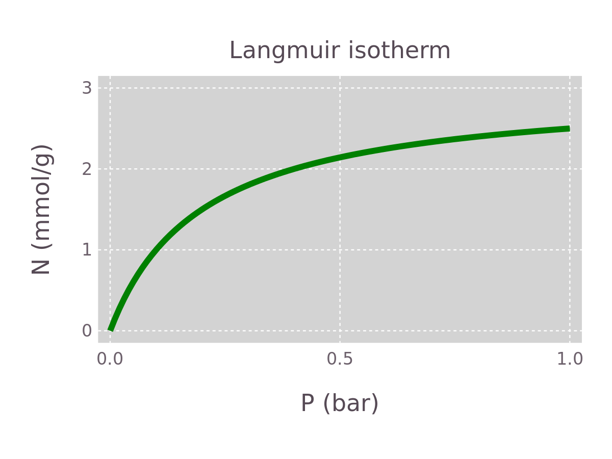
We are interested in how the parameters $M$ and $K$ affect the shape of the Langmuir equation $N(P)$. Using Gadfly, we start by plotting $N(P)$ for a given value of $K$ and $M$.

using Gadfly

# make a pretty theme
plot_theme = Theme(line_width=1mm, 
        default_color=color("green"), 
        panel_fill=color("lightgray"),
        grid_color=color("white"));

# create an array of pressures
P = linspace(0, 1)  # bar

# define parameters
M = 3.0  # (mmol/g)
K = 5.0  # (1/bar)

# plot N(P)
plot(x=P, y=M*K*P./(1+K*P), 
        Geom.line, 
        Scale.y_continuous(maxvalue=3), Scale.x_continuous(maxvalue=1),
        Guide.xlabel("P (bar)"), Guide.ylabel("N (mmol/g)"),
        Guide.title("Langmuir isotherm"),
        plot_theme)

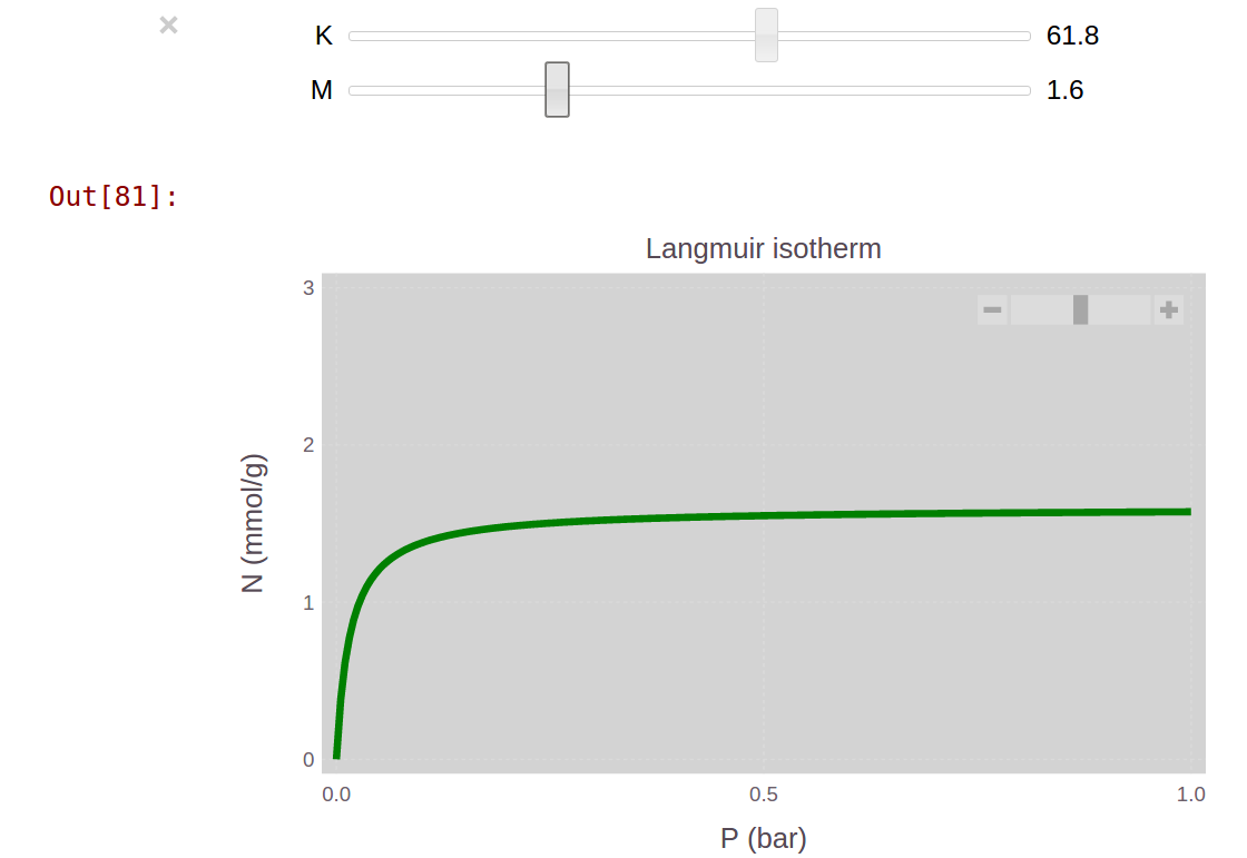
To get an idea of how $M$ and $K$ affect $N(P;K,M)$, we could manually change $M$ and $K$ in the above code and plot $N(P;K,M)$ several times. With the Julia package Interact, there is a much nicer way. The Interact package creates a slider bar with the parameters $M$ and $K$ so that we can interact with the Gadfly plot and see how $N(P;K,M)$ changes somewhat continuously.

The @manipulate macro in the Interact package creates the interactive plot with sliders to change the parameters. We can choose the parameter space of $M$ and $K$ to explore in the interactive plot. The code below explores $K \in [.1,100]$ and $M \in [1,3]$ in increments of 0.1.

using Gadfly
using Interact

@manipulate for K = .1:.1:100, M = 1.:.1:3.
    plot(x=P, y=M*K*P./(1+K*P), 
            Geom.line, 
            Scale.y_continuous(maxvalue=3), Scale.x_continuous(maxvalue=1),
            Guide.xlabel("P (bar)"), Guide.ylabel("N (mmol/g)"),
            Guide.title("Langmuir isotherm"),
            plot_theme)
end

A screenshot of the result is below.

In the IJulia Notebook, we can play with the sliders to gain insight into how the parameters $K$ and $M$ affect the shape of the Langmuir equation. The IJulia notebook with this example is here.

At a high enough pressure, $N \rightarrow M$ as the adsorption sites become filled with molecules. Intuitively, $M$ determines the value of $N$ at large pressures.

The Langmuir constant $K$ determines the initial slope of the adsorption curve at low pressures $P$ for a given $M$. In other words, it determines the pressure $P$ at which the adsorption curve starts to saturate. If we note that $N(P=K^{-1})=\frac{1}{2}M$, $K$ is inversely related to the pressure at which the adsorption sites are half-filled with molecules. Molecules with a high affinity with the surface will fill the adsorption sites at a relatively low pressure $P$; their adsorption curve will exhibit a high slope at low pressures. Therefore, a high affinity of the adsorbing molecule for the surface implies a high $K$ in the Langmuir model.