Random forests [1] are highly accurate classifiers and regressors in machine learning.
A strong advantage of random forests is interpretability; we can extract a measure of the importance of each feature in decreasing the error. One method to extract feature importance is to randomly permute a given feature and observe how the classification/regression changes. Another method is to keep track of the reduction in impurity or mean-square error, for classification or regression, respectively, that is attributed to each feature as the data falls through the trees in the forest. This is the feature importance measure implemented in scikit-learn, according to this Stack Overflow question.
This post investigates the impact of correlations between features on the feature importance measure.
Consider using a random forest as a model for a function \(f(x,y)\) of two variables \(x\in[0,1]\) and \(y\in[0,1]\):
where \(\epsilon\) is normally distributed noise.
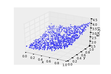
I generated data according to the above model \(f\) and trained a random forest on this data. Below is the training data set.
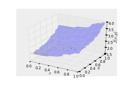
I created a grid in the \(x\)-\(y\) plane to visualize the surface learned by the random forest. It mimics the model \(f\).
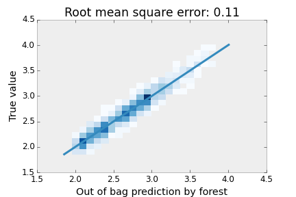
The comparison between the out of bag prediction and the true value of \(f\) in the training data is shown in the following 2D histogram. The blue diagonal line is a perfect prediction. I added a noise term \(\epsilon\) with variance 0.1, so the root mean square error from the out of bag examples is excellent.
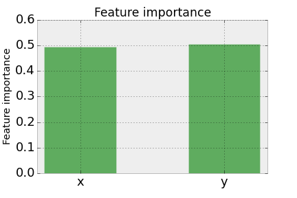
Further, the variable importance from scikit-learn gives what we’d expect; \(x\) and \(y\) are equally important in reducing the mean-square error.
Now, what happens when we introduce a third feature, \(z\), into our training data that is generated by the same underlying model \(f(x,y)\)?
Case 1: \(z\) has zero correlation with \(x\) and \(y\)
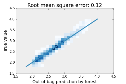
I simulated a case where \(z\) is not correlated with \(x\) or \(y\) at all by generating \(z\) as an independent, uniformly distributed number. I then trained a random forest on the feature \([x,y,z]\). The forest still performs very well on the training data, despite having an irrelevant variable thrown into the mix in my attempt to confuse the trees. Its root mean square error is increased by only 0.01 from when we trained on the feature \([x,y]\). This is another advantage of decision forests; decision trees are not so confused by irrelevant variables.
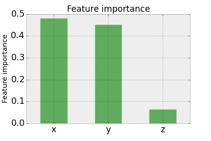
For the feature importance, the trees picked up on the fact \(z\) is irrelevant, as the trees just ignored \(z\) by not considering it for making splits.
Case 2: \(z\) is correlated with \(y\)
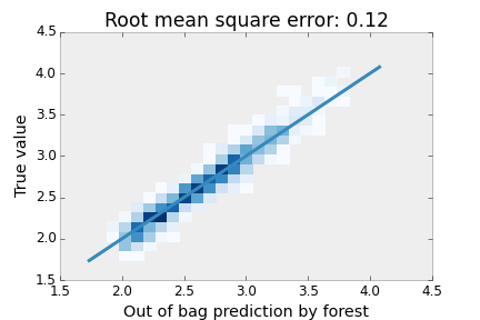
Next, in my generation of the training data, I used the same model \(f(x,y)\) but let \(z=y\) so that \(z\) and \(y\) are perfectly, positively correlated. I then trained a random forest using the feature \([x,y,z]\). Again, the forest’s prediction was very good, with the same mean square error as in Case 1.
However, when considering the feature importance, it looks very different from Case 1.
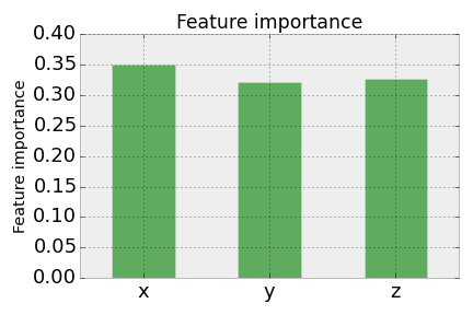
We now have that \(x\), \(y\), and \(z\) have roughly equal importance. This is intuitive, as \(x\) and \(y\) have equal importance in the model \(f\), and essentially we could write the model as \(f(x,z)=2+x+z+\epsilon\) since \(z\) is a proxy for \(y\).
Still, in some philosophical sense, \(z\) is not important at all, as we could remove \(z\) from the feature vector and get the same quality of prediction!
The IPython Notebook for this analysis can be viewed here and downloaded on Github.
[1] Breiman, L. Machine learning 2001, 45, 5-32.
comments powered by Disqus