Berkson’s paradox is a counter-intuitive result in probability and statistics. Imagine that we have two independent events A and B. By definition of independence, the conditional probability of event A given B is the same as the probability of event A:
i.e., knowing that event B occurred gives us no information about the probability that A occurred.
Berkson’s paradox is that, if we restrict ourselves to the cases where events A or B occur– where least one of the events A or B occurs– knowledge that B has occurred makes it less likely that A has occurred:1
The reason that this result is counter-intuitive is that A and B are independent events – – but they become negatively dependent on each other when we restrict ourselves to the cases that A or B occurs. We will see that Berkson’s paradox is a form of selection bias; in restricting ourselves to A or B, we ignore the cases where both A and B do not occur.
Berkson’s paradox can be used to explain the exacerbation of stereotype that the most handsome men are jerks and that the nicest men are ugly, proposed by Jordan Ellenberg in his book How Not to Be Wrong.
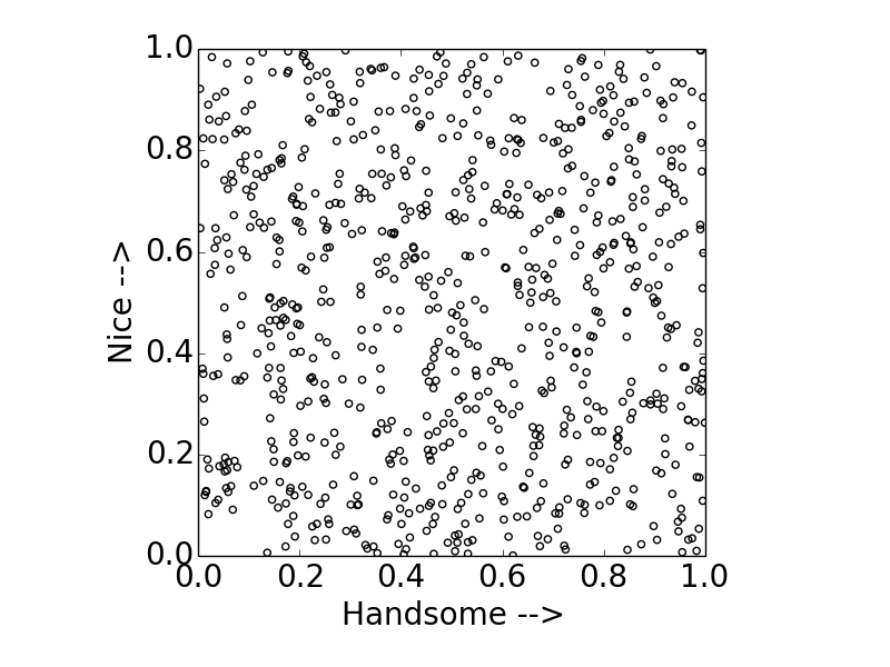
Let’s assume for the moment that looks and niceness are independent variables in the population of males so that men are randomly distributed on the looks-niceness plane:

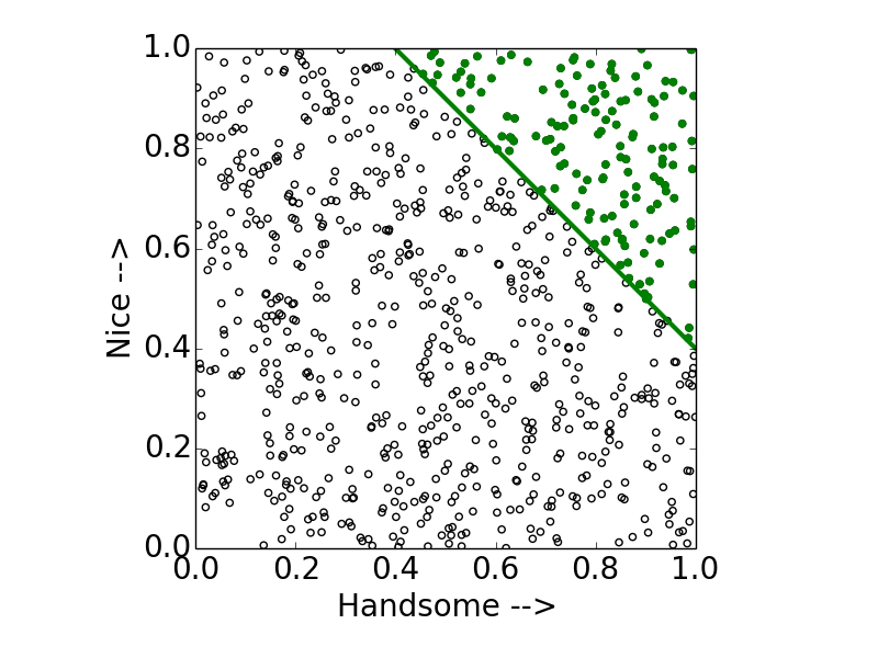
So each guy is a point in this plane. Every girl wants to date a guy in the top right corner of this plot2: a man that is both handsome and nice. However, if a guy is a jerk sometimes, she might still date him if he is really good-looking. Similarly, if a guy is really nice, she might still date him even if he is lacking in the looks category. Thus, the guys that she is willing to date are probably where:
Niceness + Handsomeness > some constant value,
the green points in the upper-right corner:

From this natural compromising behavior in her dating criterion, many of the best-looking guys that this girl dates are not so nice; many of the nicest guys she dates are not as good-looking. By restricting herself to this set of guys, she sees a negative correlation between looks and niceness, despite these two variables being independent in the population! This is Berkson’s paradox, and now you can see that this induced correlation stems from selection bias. Her dating criterion causes her to ignore the men that are decently nice, but only decently good-looking.
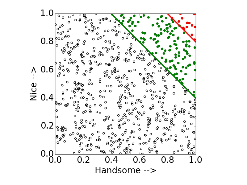
We can go one step further: maybe the guys in the very top-right corner (red points) are so nice and handsome that they will not consider dating the girl we are considering, who is just decently nice and good-looking.

Now her dating pool is even more restricted due to selection bias, and the negative correlation between good looks and niceness is even more severe.
The lesson here is that we can see spurious correlations between variables as a result of selection bias. We must think carefully about if our experiences and data collection strategies adequately sample the population in question to make sound conclusions from our observations.
The paradox is named after Joseph Berkson, who pointed out a selection bias in case-control studies to identify causal risk factors for a disease. If the control group is taken from within the hospital, a negative correlation could arise between the disease and the risk factor because of different hospitalization rates among the control and case sample.
Another example comes from the book Causality: Models, Reasoning, and Inference by Judea Pearl regarding university admissions criteria. The admissions office at a university may consider both GPA and SAT scores for admissions. Of course, the university wants students with both a high GPA and high SAT. However, a school may still admit a student with a poor GPA if he or she has a very high SAT score and admit a student with a poor SAT score if he or she compensates with a high GPA. Even if the GPA and SAT scores were independent variables, this selection bias could induce a negative correlation between GPA and SAT scores among the student body. If we change the labels on the x- and y-axes in the figures above to “GPA” and “SAT score”, the selection bias for colleges is analogous.
[1] Berkson, Joseph (June 1946). “Limitations of the Application of Fourfold Table Analysis to Hospital Data”. Biometrics Bulletin 2 (3): 47–53
1 We need 0 < P(A), P(B) < 1 for this. That is, the events have to be interesting enough that A/B do not occur with certainty or never.
2 Of course, niceness and handsomeness are [hopefully] not the only variables that a girl will consider in the guys that she dates. Please excuse this simplification.
comments powered by Disqus